学习即自动从数据集中获取最优参数的过程。
用损失函数来衡量学习的优劣
本书采用函数斜率的梯度法
机器学习、深度学习极力避免人为介入
引例
识别手写5,该如何实现?
一种方案是,先从图像中提取特征量,图像的特征量表示为向量的形式。在计算机视觉里,常采用SIFT,SURF,和HOG等,然后使用机器学习中的SVM,KNN等方法学习。
而深度学习不需要找到这个“特征量”,即直接输入数据即可。故其也被称为端到端学习。
SIFT(Scale-Invariant Feature Transform)是一种图像处理算法,用于在数字图像中寻找关键点(keypoints)并计算这些关键点的描述符(descriptor)。SIFT算法最初由David Lowe在1999年提出,并在2004年进行了改进和扩展。
SIFT算法的主要优点是其对尺度、旋转和亮度变化的鲁棒性,使其在图像配准、物体识别、图像检索等领域具有广泛的应用。SIFT算法的关键步骤包括尺度空间极值检测、关键点定位、定向分配、关键点描述和关键点匹配。
在SIFT算法中,尺度空间极值检测用于检测图像中具有不同尺度和位置的关键点。通过在不同尺度上的高斯平滑和差分操作,可以在图像中找到稳定的极值点,这些点通常对应于图像中的角点、边缘和斑点等显著特征。
关键点定位阶段对尺度空间极值点进行精确定位,排除低对比度和边缘响应不明显的点,并使用插值方法确定关键点的亚像素位置。
定向分配阶段计算每个关键点的主要方向,以便后续步骤中关键点描述子的旋转不变性。
关键点描述阶段使用关键点周围的图像梯度信息生成一个128维的描述子,该描述子能够描述关键点周围的局部外貌特征。
最后,关键点匹配阶段将两个图像的关键点进行匹配,通常使用最近邻匹配和阈值筛选来确定匹配对。
总之,SIFT算法是一种强大的图像处理算法,通过寻找图像中的关键点并计算其描述子,可以实现对图像中的特征进行鲁棒和准确的描述和匹配。
SURF(Speeded-Up Robust Features)是一种计算机视觉算法,用于在数字图像中检测和描述关键点。它是由Herbert Bay等人在2006年提出的,旨在提高SIFT算法的计算速度和匹配性能。
与SIFT算法类似,SURF算法也具有尺度不变性和旋转不变性,能够在图像中找到具有稳定特征的关键点。然而,SURF算法通过使用一种称为积分图像(integral image)的数据结构,以及一种称为快速哈尔小波(Fast-Haar wavelet)变换的方法,实现了更快的计算速度。
SURF算法的关键步骤包括构建尺度空间、检测关键点、计算关键点的描述子和关键点匹配。
在构建尺度空间阶段,SURF算法使用一种尺度空间金字塔的结构,通过对图像进行多次尺度缩放来检测不同尺度的特征。
关键点检测阶段使用Hessian矩阵的行列式来检测尺度空间中的极值点,这些极值点被认为是图像中的关键点。
关键点描述阶段利用关键点周围的局部图像区域,通过计算Haar小波响应来生成一个描述子向量。这个描述子向量包含了关键点周围区域的梯度方向和强度信息。
最后,关键点匹配阶段使用一种快速的最近邻算法(例如KD树)来将两个图像的关键点进行匹配,以找到相似的特征点。
总的来说,SURF算法是一种高效、快速且具有良好性能的特征提取和匹配算法。它在计算机视觉中广泛应用于目标检测、图像配准、三维重建等领域。
HOG(Histogram of Oriented Gradients)是一种用于目标检测和图像识别的特征描述算法。HOG算法最初由Navneet Dalal和Bill Triggs在2005年提出,并在物体检测领域取得了很大的成功。
HOG算法的基本思想是将图像中的局部区域转换为特征向量,这些特征向量能够描述图像中的边缘和纹理信息。HOG算法对图像的梯度方向进行统计,生成一个直方图来表示图像中不同方向上的梯度分布。
HOG算法的主要步骤如下:
图像预处理:将输入图像进行预处理,通常包括灰度化、归一化和对比度增强等操作。
计算梯度:计算图像中每个像素点的梯度幅值和方向,可以使用Sobel等算子进行梯度计算。
划分图像区域:将图像划分为多个小的局部区域(cells),每个局部区域包含多个像素点。
计算局部直方图:对每个局部区域内的像素点,统计其梯度方向的分布情况,生成一个局部直方图。
归一化直方图:对于相邻的若干个局部区域,将它们的局部直方图进行归一化,以增强对光照变化的鲁棒性。
特征向量描述:将所有归一化的局部直方图连接起来,形成一个全局的特征向量,用于表示整个图像。
最终,HOG算法通过计算图像中不同位置上的特征向量之间的相似性,实现目标检测和图像识别任务。通常使用支持向量机(SVM)等分类器来训练和识别目标。
HOG算法在人脸检测、行人检测等领域取得了很好的效果,并且相对于其他特征描述算法,HOG算法具有计算简单、鲁棒性强的优点。
深度学习需要提高
泛化能力
避免过拟合
损失函数:
是评价神经网络性能恶劣程度的指标。
- 均方误差函数
$$E=\frac{1}{2} \sum_k{(y_k-t_k)^2}$$$$y_k表示输出,t_k表示监督数据,k表示数据维度$$
1
2
3
4
5
6
7
8
9
10
11
|
import numpy as np

from sklearn.metrics import mean_squared_error

t=[0  ,0   ,1  ,0  ,0   ,0  ,0  ,0  ,0  ,0  ]

y=[0.1,0.05,0.6,0.0,0.05,0.1,0.0,0.1,0.0,0.0]

print(mean_squared_error(np.array(y),np.array(t)))
|
0.019500000000000007
- 交叉熵误差
$$ E=-\sum_k{t_k\log{y_k}} $$$$t_k采用one-hot表示$$
该式只计算了正确标签输出的自然对数。误差的值由正确标签对应的输出结果决定的。
1
2
3
4
5
6
7
8
9
10
11
12
13
|
def cross_entropy_error(y,t):

    delta=1e-7

    return -np.sum(t*np.log(y+delta))

t=[0,0,1,0,0,0,0,0,0,0]

y=[0.1,0.05,0.6,0.0,0.05,0.1,0.0,0.1,0.0,0.0]

print(cross_entropy_error(np.array(y),np.array(t)))
|
0.510825457099338
1
2
3
4
5
|
y=[0.1,0.05,0.1,0.0,0.05,0.1,0.0,0.6,0.0,0.0]

print(cross_entropy_error(np.array(y),np.array(t)))
|
2.302584092994546
mini-batch
若全部计算损失,则耗费资源过大。故一般选择一部分,作为全部数据的近似(注意考虑分布,方差,均值等因素,尽量保持一致)。用这一部分数据学习。
1
2
3
4
5
6
7
8
9
10
11
12
13
14
15
|
import sys, os
import numpy as np
from source.dataset.mnist import load_mnist
(x_train,t_train),(x_test,t_test)=load_mnist(normalize=True,one_hot_label=True)
print(x_train.shape)
print(t_train.shape)
|
(60000, 784)
(60000, 10)
1
2
3
4
5
6
7
8
9
10
11
12
13
|
train_size=x_train.shape[0]
batch_size=10
batch_mask=np.random.choice(train_size,batch_size)
x_batch=x_train[batch_mask]
t_batch=t_train[batch_mask]
|
1
2
3
4
5
6
7
8
9
10
11
12
13
14
15
|
def cross_entropy_error(y,t):
if y.ndim == 1:
t=t.reshape(1,t.size)
y=y.reshape(1,y.size)
batch_size = y.shape[0]
return -np.sum(t*np.log(y+1e-7))/batch_size
|
在计算机科学和数值计算中,由于浮点数的精度限制,当一个数值非常接近于零时,可能会出现数值误差问题。在这种情况下,对一个非常接近零的数值取对数时,可能会遇到无穷大或NaN(不是一个数字)的结果。
为了避免这种情况,通常会在取对数之前,将待取对数的数值加上一个很小的常数(通常是类似1e-7这样的小数),以确保数值不会非常接近零。这样可以防止数值误差导致的无穷大或NaN的结果,并且得到一个合理的数值。
在np.log(y+1e-7) 中的1e-7就是为了避免y值非常接近零时产生数值误差。通过将1e-7添加到y上,可以确保y+1e-7不会非常接近零,从而避免了数值误差问题。
1
2
3
4
5
6
7
8
9
10
11
12
13
14
15
16
17
18
19
|
"""
def cross_entropy_error(y,t):
if y.ndim == 1:
t=t.reshape(1,t.size)
y=y.reshape(1,y.size)
batch_size = y.shape[0]
return -np.sum(t*np.log(y[np.arrange(batch_size),t]+1e-7))/batch_size
"""
|
损失函数意义
不能使用识别精度作为指标,因为以它作为指标,很多地方导数都会变为0从而无法更新参数
使用损失函数作为指标,可以根据参数变化计算损失函数,从而得出导数。
因为识别精度有可能是,而且经常是离散的点,故1.中导数很多地方都是0
同样原因,之前感知机的激活函数一般选用连续的值,即sigmoid函数,而不用阶跃函数。
数值计算
导数实现
不用导数的定义式,因为 $\delta x$ 太小会引入舍入误差。
使用中心差分,而不用前向差分。
1
2
3
4
5
6
7
8
9
|
def numerical_diff(f,x):
h=1e-4
return (f(x+h)-f(x-h))/(2*h)
|
1
2
3
4
5
6
7
8
9
10
11
12
13
14
15
16
17
18
19
20
21
22
23
24
25
26
27
28
29
30
31
|
def function_1(x):
return 0.01*x**2+0.1*x
import numpy as np
import matplotlib.pylab as plt
x=np.arange(0.0,20.0,0.1)
y=function_1(x)
plt.xlabel('x')
plt.ylabel('f(x)')
plt.plot(x,y)
plt.show()
print(numerical_diff(function_1,5))
print(numerical_diff(function_1,10))
|
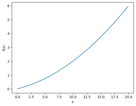
0.1999999999990898
0.2999999999986347
偏导实现
$$f(x_0,x_1)=x_0^2+x_1^2$$
1
2
3
4
5
6
7
8
9
10
11
12
13
14
15
16
17
18
19
|
def function_2(x):
return x[0]**2.0+x[1]**2.0
def function_tmp1(x0):
return x0*x0+4.0**2.0
def function_tmp2(x1):
return 3.0**2.0 + x1*x1
print(numerical_diff(function_tmp1,(3.0)))
print(numerical_diff(function_tmp2,(4.0)))
|
6.00000000000378
7.999999999999119
梯度实现
1
2
3
4
5
6
7
8
9
10
11
12
13
14
15
16
17
18
19
20
21
22
23
24
25
26
27
28
29
30
31
32
33
34
35
36
37
38
39
|
def numerical_gradient(f,x):
h = 1e-4
grad=np.zeros_like(x)
for idx in range(x.size):
tmp_val = x[idx]
x[idx]=float(tmp_val) + h
fxh1=f(x)
x[idx]=float(tmp_val) - h
fxh2=f(x)
grad[idx]=(fxh1 - fxh2)/ (2*h)
x[idx]=tmp_val
return grad
|
1
2
3
4
5
6
7
|
print(numerical_gradient(function_2, np.array([3.0,4.0])))
print(numerical_gradient(function_2, np.array([0.0,2.0])))
|
[6. 8.]
[0. 4.]
注意一点,梯度只会指向函数值下降的地方,而不是最低的地方。即只会找到极值,而不是最值。
1
2
3
4
5
6
7
8
9
10
11
12
13
14
15
16
17
|
def gradient_descent(f,init_x,lr=0.01,step_num=100):
x=init_x
for i in range(step_num):
grad=numerical_gradient(f,x)
x-=lr*grad
return x
|
1
2
3
4
5
6
7
8
9
10
11
12
13
14
15
16
17
|
def function_2(x):
return np.sum(x**2)
init_x=np.array([-3.0,4.0])
print(gradient_descent(function_2,init_x=init_x,lr=0.1,step_num=100))
print(gradient_descent(function_2,init_x=init_x,lr=0.1,step_num=10))
print(gradient_descent(function_2,init_x=init_x,lr=10.0,step_num=100))
|
[-6.11110793e-10 8.14814391e-10]
[-6.56175217e-11 8.74900290e-11]
[-9.70516708e+12 1.29488926e+13]
学习率这种属于超参数,是人工设定。一般需要尝试多个值,找到合适的参数。
1
2
3
4
5
6
7
8
9
10
11
12
13
14
15
16
17
18
19
20
21
22
23
24
25
26
27
28
29
30
31
32
33
34
35
36
37
38
39
40
41
42
43
44
45
46
47
48
49
|
import sys,os
import numpy as np
from source.common.functions import softmax, cross_entropy_error
from source.common.gradient import numerical_gradient
class simpleNet:
def __init__(self):
self.W = np.random.randn(2,3)
def predict (self, x):
return np.dot(x,self.W)
def loss(self,x,t):
z=self.predict(x)
y=softmax(z)
loss=cross_entropy_error(y,t)
return loss
net = simpleNet()
print(net.W)
x=np.array([0.6,0.9])
p=net.predict(x)
print(p)
|
[[ 0.10575028 -0.12302507 0.67452961]
[-0.65135332 0.12114118 0.91331758]]
[-0.52276782 0.03521202 1.22670359]
1
2
3
4
5
6
7
8
9
|
print(np.argmax(p))
t=np.array([0,1,0])
net.loss(x,t)
|
2
1.5819330169514783
1
2
3
4
5
6
7
8
9
10
11
|
def f(W):
return net.loss(x,t)
dW=numerical_gradient(f,net.W)
print(dW)
|
[[ 0.07059899 -0.47665343 0.40605444]
[ 0.10589848 -0.71498015 0.60908166]]
学习算法的实现
学习步骤如下:
mini-batch
计算梯度
更新参数
重复 1.
1
2
3
4
5
6
7
8
9
10
11
12
13
14
15
16
17
18
19
20
21
22
23
24
25
26
27
28
29
30
31
32
33
34
35
36
37
38
39
40
41
42
43
44
45
46
47
48
49
50
51
52
53
54
55
56
57
58
59
60
61
62
63
64
65
66
67
68
69
70
71
72
73
74
75
76
77
78
79
80
81
82
83
84
85
86
87
88
89
90
91
92
93
94
95
96
97
98
99
100
101
102
103
104
105
106
107
108
109
110
111
112
113
114
115
116
117
118
119
120
121
122
123
124
125
126
127
128
129
|
import sys, os
sys.path.append(os.pardir)
from source.common.functions import *
from source.common.gradient import numerical_gradient
class TwoLayerNet:
def __init__(self, input_size, hidden_size, output_size, weight_init_std=0.01):
self.params = {}
self.params['W1'] = weight_init_std * np.random.randn(input_size, hidden_size)
self.params['b1'] = np.zeros(hidden_size)
self.params['W2'] = weight_init_std * np.random.randn(hidden_size, output_size)
self.params['b2'] = np.zeros(output_size)
def predict(self, x):
W1, W2 = self.params['W1'], self.params['W2']
b1, b2 = self.params['b1'], self.params['b2']
a1 = np.dot(x, W1) + b1
z1 = sigmoid(a1)
a2 = np.dot(z1, W2) + b2
y = softmax(a2)
return y
def loss(self, x, t):
y = self.predict(x)
return cross_entropy_error(y, t)
def accuracy(self, x, t):
y = self.predict(x)
y = np.argmax(y, axis=1)
t = np.argmax(t, axis=1)
accuracy = np.sum(y == t) / float(x.shape[0])
return accuracy
def numerical_gradient(self, x, t):
loss_W = lambda W: self.loss(x, t)
grads = {}
grads['W1'] = numerical_gradient(loss_W, self.params['W1'])
grads['b1'] = numerical_gradient(loss_W, self.params['b1'])
grads['W2'] = numerical_gradient(loss_W, self.params['W2'])
grads['b2'] = numerical_gradient(loss_W, self.params['b2'])
return grads
def gradient(self, x, t):
W1, W2 = self.params['W1'], self.params['W2']
b1, b2 = self.params['b1'], self.params['b2']
grads = {}
batch_num = x.shape[0]
a1 = np.dot(x, W1) + b1
z1 = sigmoid(a1)
a2 = np.dot(z1, W2) + b2
y = softmax(a2)
dy = (y - t) / batch_num
grads['W2'] = np.dot(z1.T, dy)
grads['b2'] = np.sum(dy, axis=0)
da1 = np.dot(dy, W2.T)
dz1 = sigmoid_grad(a1) * da1
grads['W1'] = np.dot(x.T, dz1)
grads['b1'] = np.sum(dz1, axis=0)
return grads
|
1
2
3
4
5
6
7
8
9
10
11
12
13
14
15
16
17
18
19
20
21
22
23
24
25
26
27
28
29
30
31
32
33
34
35
36
37
38
39
40
41
42
43
44
45
46
47
48
49
50
51
52
53
54
55
56
57
58
59
60
61
62
63
64
65
66
67
68
69
70
71
72
73
74
75
76
77
78
79
80
81
82
83
84
85
86
87
88
89
90
91
92
93
94
95
96
97
98
99
100
101
102
103
104
105
106
107
108
109
|
import sys, os
sys.path.append(os.pardir)
import numpy as np
import matplotlib.pyplot as plt
from source.dataset.mnist import load_mnist
from source.ch04.two_layer_net import TwoLayerNet
(x_train, t_train), (x_test, t_test) = load_mnist(normalize=True, one_hot_label=True)
network = TwoLayerNet(input_size=784, hidden_size=50, output_size=10)
iters_num = 10000
train_size = x_train.shape[0]
batch_size = 100
learning_rate = 0.1
train_loss_list = []
train_acc_list = []
test_acc_list = []
iter_per_epoch = max(train_size / batch_size, 1)
for i in range(iters_num):
batch_mask = np.random.choice(train_size, batch_size)
x_batch = x_train[batch_mask]
t_batch = t_train[batch_mask]
grad = network.gradient(x_batch, t_batch)
for key in ('W1', 'b1', 'W2', 'b2'):
network.params[key] -= learning_rate * grad[key]
loss = network.loss(x_batch, t_batch)
train_loss_list.append(loss)
if i % iter_per_epoch == 0:
train_acc = network.accuracy(x_train, t_train)
test_acc = network.accuracy(x_test, t_test)
train_acc_list.append(train_acc)
test_acc_list.append(test_acc)
print("train acc, test acc | " + str(train_acc) + ", " + str(test_acc))
markers = {'train': 'o', 'test': 's'}
x = np.arange(len(train_acc_list))
plt.plot(x, train_acc_list, label='train acc')
plt.plot(x, test_acc_list, label='test acc', linestyle='--')
plt.xlabel("epochs")
plt.ylabel("accuracy")
plt.ylim(0, 1.0)
plt.legend(loc='lower right')
plt.show()
|
train acc, test acc | 0.09863333333333334, 0.0958
train acc, test acc | 0.7992, 0.8057
train acc, test acc | 0.8787833333333334, 0.8825
train acc, test acc | 0.9001166666666667, 0.9031
train acc, test acc | 0.9101166666666667, 0.9111
train acc, test acc | 0.9163833333333333, 0.9195
train acc, test acc | 0.9212333333333333, 0.9224
train acc, test acc | 0.9265333333333333, 0.9276
train acc, test acc | 0.9294, 0.9307
train acc, test acc | 0.9323166666666667, 0.9333
train acc, test acc | 0.9355333333333333, 0.9358
train acc, test acc | 0.9381, 0.9389
train acc, test acc | 0.93975, 0.9407
train acc, test acc | 0.9418166666666666, 0.9419
train acc, test acc | 0.9431166666666667, 0.9421
train acc, test acc | 0.9453666666666667, 0.9446
train acc, test acc | 0.9470833333333334, 0.9461
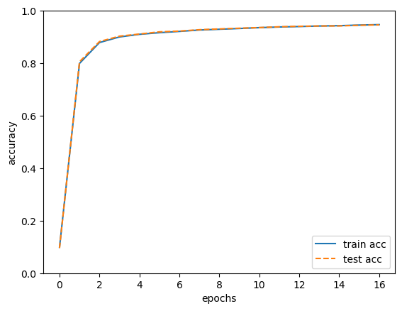
这里的epochs代表所有数据都被使用过一次时的更新次数。
e.g 10000笔数据,mini-batch 是 100,则一个epoch就是 100次。
注意到train和test的识别精度曲线基本重合,故可以认没有发生过拟合现象